1. Exploring Matplotlib Internals: Figures, Axes, and More#
In this section#
We will learn how to create figures consistent with the rest of the document. A consistent figure is one that has the same font properties, proper size, and resolution. We will use the rich library to inspect matplotlib objects when exploring the properties. And learn a lot about matplotlib Figure and Axis objects.
Figure#
According to the Oxford English Dictionary, the word “figure” has several meanings.
Figure
n 1. a number or numerical symbol. 2. a geometric or decorative shape defined by one or more lines. 3. a diagram or illustrative drawing.
v 1. play an important part. 2. calculate arithmetically. 3. (figure someone/thing out) understand someone or something. 4. think; consider.
In many cases, figures do not exist in isolation, they appear in the text, presentation, or webpage.
Have you ever noticed that in many places, figures look alien? They are very different than the rest of the environment they are placed in.
Here is an example of such a figure:
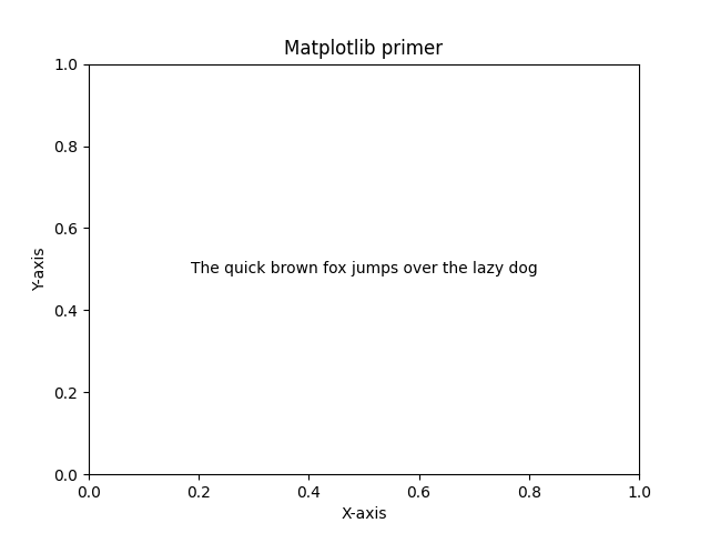
Figure 1. A figure created with Matplotlib default settings.#
The content is pixelated and hard to read. The figure below looks better.
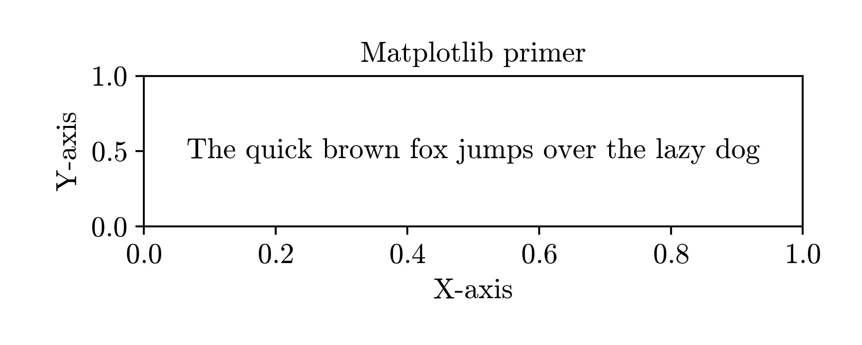
Figure 2. A figure with adjusted shape size and font size.#
There is still a tiny misalignment regarding fonts with the rest of the webpage. But this is quite a complex problem to align. Matplotlib excels in generating high-quality figures.
In the context of this workshop, a Figure is an object with physical properties like width and height. It also contains axes, lines, fonts, and legends.
You don’t need to be a designer to create pretty figures; start with the right Figure size and font properties. This should improve the overall integrity of the documents because the plots will look like they belong to the rest of the document.
For example, here is a screenshot of a simple HTML page we’ll create in the first part of the workshop. Looks like LaTeX, right? But it is not; it is just an HTML page with an appropriately configured Matplotlib figure.
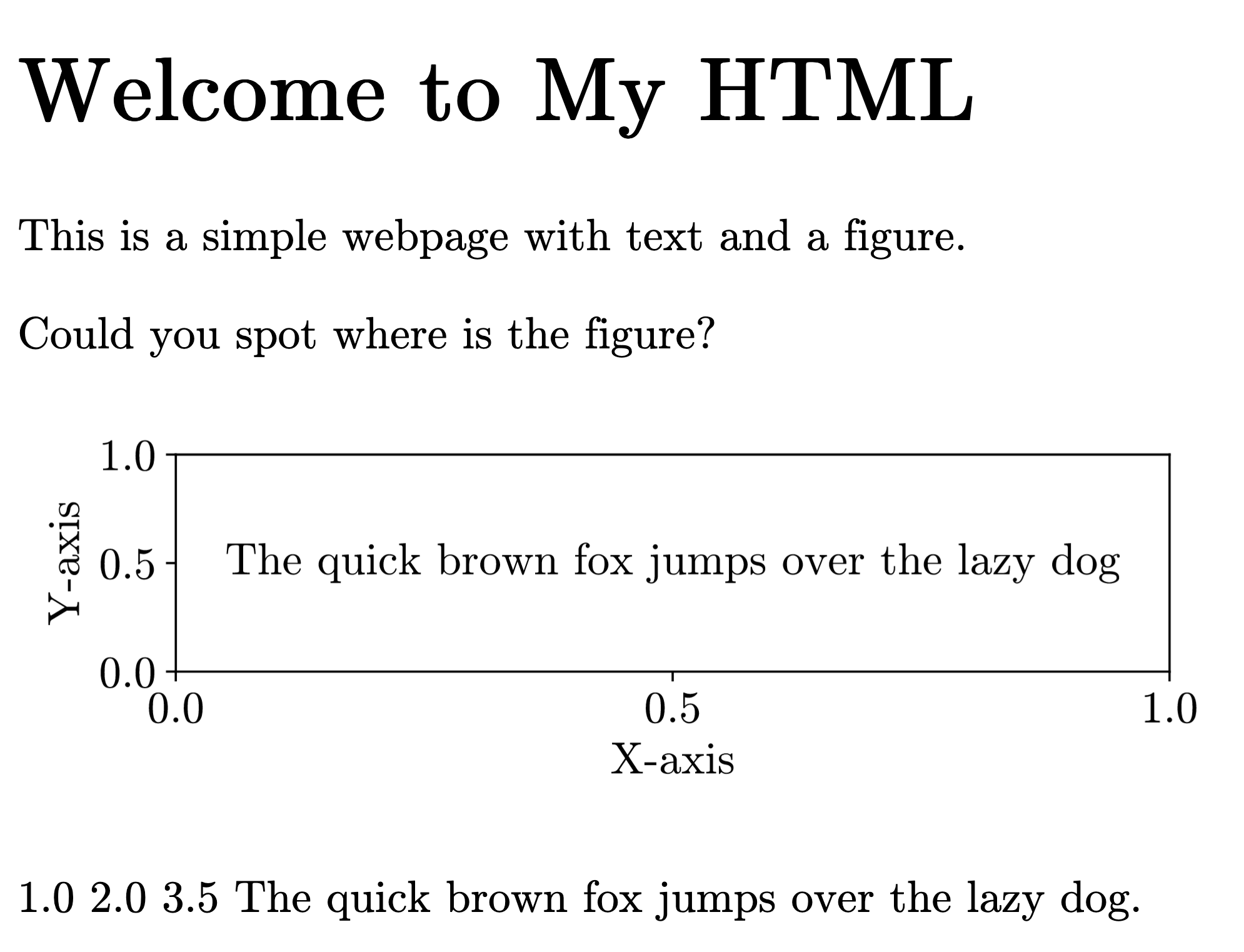
Figure 3. Plain HTML provides full control over the document’s look, making it easy to match the font properties of the figure and the webpage.#
Part 1: Working with Figures in Matplotlib#
The figure is the central object of this workshop. In Matplotlib, the figure is the top-level object for all the plot elements. Mastering the figure object is crucial to creating high-quality visualizations that look nice in the context of the document.
The goal of Part 1 is to create a document with a figure using the same font properties as the rest of the content.
TODO: link to the jupyter notebook.
Matplotlib Documentation Pointers:
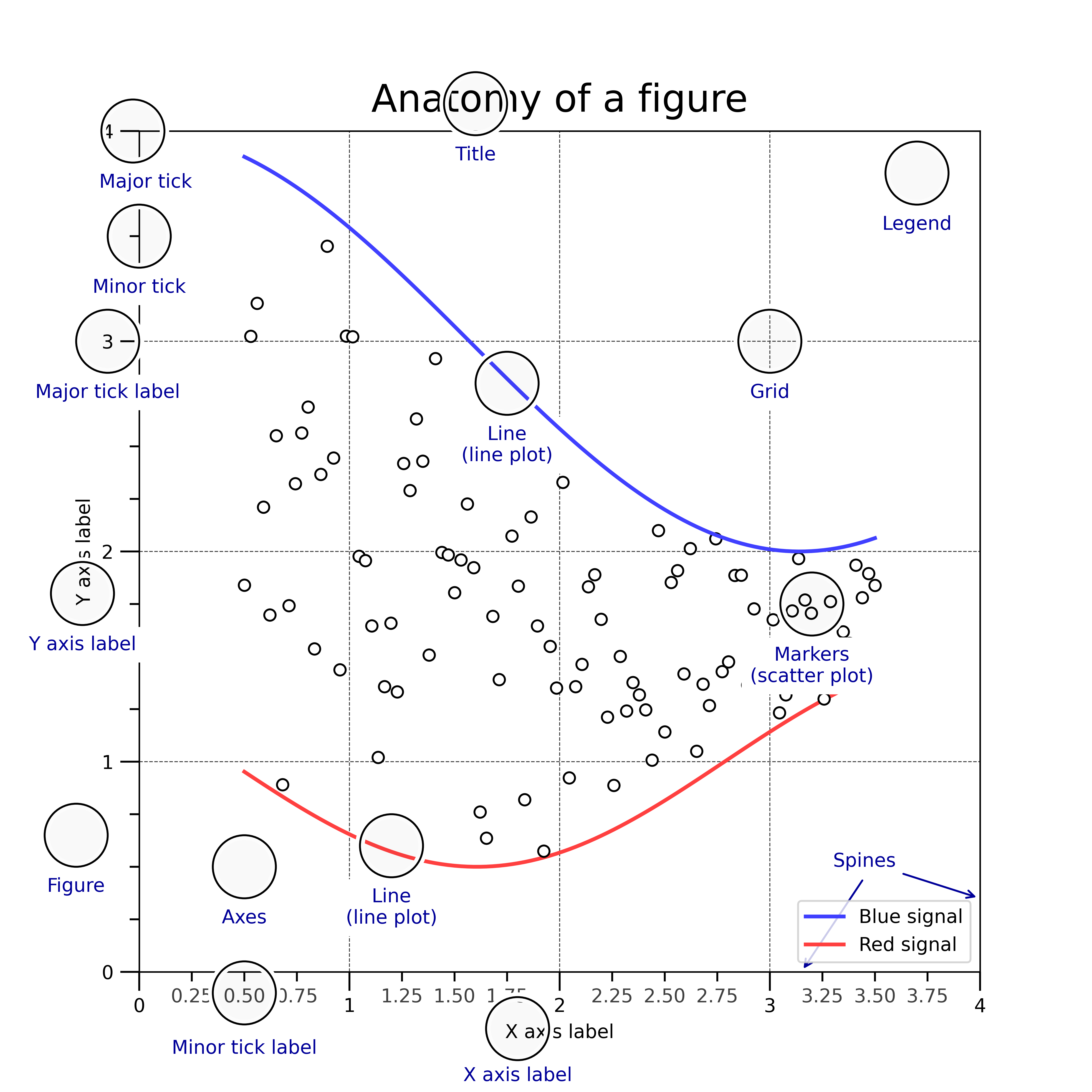
Anatomy of a Figure#
Axes#
Axes != Axis. Here are some doc links:
When you create a figure with plt.figure(), it is empty. You need to add axes to it to start plotting. plt.subplots() is another very common way to create a figure with axes in one go.
But there is a catch. The Figure is the top-level object, but the Axes object is the one that holds the data and almost all visual elements of the plot. When we plot something, we are actually adding attributes to the Axes object.
But how do I know that?
That’s where debugging techniques come in handy.
One of my favorite tools for exploring objects is the rich library. Inspect function is a fantastic debug aid that can be used to explore objects in Python. Take a figure object for an example:
>>> from matplotlib import pyplot as plt
>>> from rich import inspect
>>> fig = plt.figure()
>>> inspect(fig)
╭─────────────────────── <class 'matplotlib.figure.Figure'> ────────────────────────╮
│ The top level container for all the plot elements.                                │
│                                                                                   │
│ ╭───────────────────────────────────────────────────────────────────────────────╮ │
│ │ <Figure size 1280x960 with 0 Axes>                                            │ │
│ ╰───────────────────────────────────────────────────────────────────────────────╯ │
│                                                                                   │
│           artists = []                                                            │
│              axes = []                                                            │
│              bbox = <matplotlib.transforms.TransformedBbox object at 0x132cf3a40> │
│       bbox_inches = Bbox([[0.0, 0.0], [6.4, 4.8]])                                │
│            canvas = FigureCanvas object 0x132e56b50 wrapping NSView 0x1437bb380   │
│           clipbox = None                                                          │
│               dpi = 200.0                                                         │
│   dpi_scale_trans = <matplotlib.transforms.Affine2D object at 0x132e59ca0>        │
│           figbbox = <matplotlib.transforms.TransformedBbox object at 0x132cf3a40> │
│            figure = <Figure size 1280x960 with 0 Axes>                            │
│           frameon = True                                                          │
│            images = []                                                            │
│           legends = []                                                            │
│             lines = []                                                            │
│         mouseover = False                                                         │
│            number = 2                                                             │
│             patch = <matplotlib.patches.Rectangle object at 0x132e59be0>          │
│           patches = []                                                            │
│             stale = False                                                         │
│      sticky_edges = _XYPair(x=[], y=[])                                           │
│           subfigs = []                                                            │
│       subplotpars = <matplotlib.figure.SubplotParams object at 0x132e59b50>       │
│ suppressComposite = None                                                          │
│             texts = []                                                            │
│       transFigure = <matplotlib.transforms.BboxTransformTo object at 0x132e5b9e0> │
│    transSubfigure = <matplotlib.transforms.BboxTransformTo object at 0x132e5b9e0> │
│            zorder = 0                                                             │
╰───────────────────────────────────────────────────────────────────────────────────╯
Or you could call inspect with methods set to True (inspect(fig, methods=True)) to list all the attributes and methods of the object. The output is parsed and formatted by the rich library, which makes it easy to read and understand.
>>> from matplotlib import pyplot as plt
>>> from rich import inspect
>>> fig, ax = plt.subplots()
>>> inspect(ax)
╭──────────────────────────────── <class 'matplotlib.axes._axes.Axes'> ─────────────────────────────────╮
│ An Axes object encapsulates all the elements of an individual (sub-)plot in                           │
│ a figure.                                                                                             │
│                                                                                                       │
│ ╭───────────────────────────────────────────────────────────────────────────────────────────────────╮ │
│ │ <Axes: >                                                                                          │ │
│ ╰───────────────────────────────────────────────────────────────────────────────────────────────────╯ │
│                                                                                                       │
│                     artists = <Axes.ArtistList of 0 artists>                                          │
│                        axes = <Axes: >                                                                │
│                      axison = True                                                                    │
│                        bbox = <matplotlib.transforms.TransformedBbox object at 0x1330ce3c0>           │
│                   callbacks = <matplotlib.cbook.CallbackRegistry object at 0x1330cf8f0>               │
│                  child_axes = []                                                                      │
│                     clipbox = None                                                                    │
│                 collections = <Axes.ArtistList of 0 collections>                                      │
│                  containers = []                                                                      │
│                     dataLim = Bbox([[inf, inf], [-inf, -inf]])                                        │
│                      figure = <Figure size 1280x960 with 1 Axes>                                      │
│                   fmt_xdata = None                                                                    │
│                   fmt_ydata = None                                                                    │
│ ignore_existing_data_limits = True                                                                    │
│                      images = <Axes.ArtistList of 0 images>                                           │
│                     legend_ = None                                                                    │
│                       lines = <Axes.ArtistList of 0 lines>                                            │
│                   mouseover = False                                                                   │
│                        name = 'rectilinear'                                                           │
│                       patch = <matplotlib.patches.Rectangle object at 0x13309cc80>                    │
│                     patches = <Axes.ArtistList of 0 patches>                                          │
│                      spines = <matplotlib.spines.Spines object at 0x1330ce780>                        │
│                       stale = False                                                                   │
│                sticky_edges = _XYPair(x=[], y=[])                                                     │
│                      tables = <Axes.ArtistList of 0 tables>                                           │
│                       texts = <Axes.ArtistList of 0 texts>                                            │
│                       title = Text(0.5, 1.0, '')                                                      │
│            titleOffsetTrans = <matplotlib.transforms.ScaledTranslation object at 0x13309ff80>         │
│                   transAxes = <matplotlib.transforms.BboxTransformTo object at 0x132d2a570>           │
│                   transData = <matplotlib.transforms.CompositeGenericTransform object at 0x1330ceb70> │
│                 transLimits = <matplotlib.transforms.BboxTransformFrom object at 0x1330ce150>         │
│                  transScale = <matplotlib.transforms.TransformWrapper object at 0x1330ce810>          │
│            use_sticky_edges = True                                                                    │
│                     viewLim = Bbox([[0.0, 0.0], [1.0, 1.0]])                                          │
│                       xaxis = <matplotlib.axis.XAxis object at 0x1330cef00>                           │
│                       yaxis = <matplotlib.axis.YAxis object at 0x1330cd370>                           │
│                      zorder = 0                                                                       │
╰───────────────────────────────────────────────────────────────────────────────────────────────────────╯
With this you are equipped to start exploring any codebase and understand how it works. We’ll do it with Matplotlib.
Practice#
Let’s jump into the code and start exploring Matplotlib. https://github.com/Kislovskiy/ChartCraftHub/blob/trunk/src/chartcrafthub/chapter_1_0.ipynb
List of Exercises#
Exercise 1#
Description:
Use the editor of your choice: HTML, GoogleDocs, Word, Pages… Create a page that looks like it was created with LaTeX.
Exercise 2#
Description
Following the chapter_2_1.ipynb create a code to generate a figure below.
Summary#
We’ve learned about two most powerful objects in Matplotlib: Figure and Axes. They are always coming together and are the foundation of any plot.
There are two most important things I want you to remember:
First:#
from matplotlib import pyplot as plt
import matplotlib

matplotlib.rcParams.update(
    {
        "font.family": "sans-serif",
        "font.sans-serif": "cmr10",
        "font.size": 16,
        "axes.formatter.use_mathtext": True,
    }
)

fig, ax = plt.subplots(figsize=(3, 3), dpi=300)
ax.text(x=0.5, y=0.5, s="Hello World!", ha="center", va="center")
ax.set_xlabel("Hello World!")
fig.savefig("results/hello_world.svg")
plt.show()
Note
Note: that the font should be installed on your system. One gotcha is that matplotlib stores fonts available on your system in .matplotlib folder in your home directory. To see the newly installed font, you need to remove the font cache file.
~ ❯❯❯ la .matplotlib
Permissions Size User       Date Modified Name
.rw-r--r--@ 140k kislovskiy 15 Mar 22:11  fontlist-v330.json
Second:#
from matplotlib import pyplot as plt
from rich import inspect

fig, ax = plt.subplots()
inspect(ax, methods=True)